Making recipes
Each ETA recipes consitis of Virtual Instruments , Script Panel and optionally Parameter.
Here is the workflow of building an ETA recipe, if you are not using ready-made ones.
Add Virtual Instruments to perform analysis
Click the Virtual Instruments button on the main screen to create a new analysis routine and open it in the Instrument Designer.
This is the place where you define how exactly the ETA backend analyses your data.
You create an analysis instrument in two steps:
- Create a state diagram (https://en.wikipedia.org/wiki/State_diagram) through which the program transitions that covers all relevant states that your analysis undergoes (left-hand side of the instrument)
- Create some (simple) code to define what actions should be performed upon one (or several) specific transitions (right-hand side of the Instrument Designer)
- Add your time-tagger in Virtual Instruments
Make an RFILE in the action panel.
Specify the name for RFILE, assign the physically available channels and the number of marker channels.
TODO: explain how to do it with PicoQuant HydraHarp400
- We can use the state diagram described above to analyze a time tag file with two channels in a start-stop manner. For this we need to add a histogram into which we save the time differences between events. We also need a clock to record these time differences. Both these entities can be created with the help of the “Create” menu in the top bar of the Instrument Designer. You can also directly type into the code panel:
HISTOGRAM(name, (number_of_bins, bin_size))
CLOCK(name)
From this point on I will assume that the state diagram is labelled as follows:
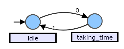
I will also assume the histogram is named h1 and the clock is named c1. We will define actions so that we use channel 0 as the start channel and channel 1 as the stop channel. (Note, that this analysis will not record time differences between closest events, since the start is not reset if a second event occurs on channel 0 before an event occurs on channel 1. See Section “Coincidence Measurements”)
To define an action you select a transition after which you would like the action to happen.
With this transition selected press SHIFT + T (think: Trigger). You will see state_at_arrow_tail–list_of_channel_numbers–>state_at_arrow_head followed by a colon (:) appear in the code on the right-hand side. By using indentations you can now specify actions that should be performed upon completion of the transition. In case of a start-stop measurement we want to start the clock when there is an event on channel 0. We therefore write:
idle--0-->taking_time:
  c1.start()
To stop the clock and record the time difference in our histogram we write:
taking_time--1-->idle:
  c1.stop()
  h1.record(c1)
- Additional Info:
- States can loop to themselves.
- Labels can be written underneath the state (e.g. when they become too long to fit) with SHIFT + M (think: Mark)
TODO:explain the following and add more functions
COINCIDENCE()
TABLE()
Allowed action definitions
TODO: Insert graph
a--1-->b:
  action1
a--2,4-->b:
  action2
b: #involves all transitions arriving to b
  action3
TODO: explain all the analysis actions
start(clock)
start(c1)
Start a clock labeled c1.

stop(clock)
stop(c1)
Stop a clock labeled c1.

emit(channel_number,waittime_ps,period_ps,repeat)
emit(2,10)
Emit signal to a channel 2 after 10 picoseconds.

record(histogram,clock)
record(h1,c1)
Record the time interval on clock c1 to histogram h1.

fill(coincidence,slot_number)
fill(coinci1,1)
Record coincidence event on slot 1 of coincidence tool coinci1.

clear(coincidence,slot_number)
clear(coinci1,1)
Clear coincidence event of coincidence tool coinci1.
Add Script Panel
In the Script Panel you tell ETA to run your analysis and define what happens with the result.
A minimum example that saves the data as an Origin-compatitable *.txt file looks as follows:
import numpy as np
result =eta.run(eta.clip(filename)) #tell ETA to run the analysis on "filename"
histogram = result["h1"] #get the table from result
np.savetxt("h1.txt",histogram) #save the txt file for the histogram
eta.send("processing succeed.") #display message on GUI popup
Instead or in addition to saving a file, the data can be displayed/treated in various ways.
In the following example dash from plotly is used to create an interactive graph from a histogram.
app is a Dash object which gets modified with the style configurations.
eta.display(app) is used for displaying the Dash on the GUI side.
import numpy as np
import dash
import dash_core_components as dcc
import dash_html_components as html
import plotly.graph_objs as go
result =eta.run(eta.clip(filename))
histogram = result["h1"] #get the table from result

app = dash.Dash()
app.layout = html.Div(children=[
    html.H1(children='Result from ETA'),
    html.P(children='+inf_bin={}'.format(inf)),
    dcc.Graph(
        id='example-graph',
        figure={
            'data': [
                {'x': np.arange(histogram.size), 'y': histogram, 'type': 'bar', 'name': 'SF'},
            ],
            'layout': {
                'title': expname
            }
        }
    )
])

eta.display(app)
Please refer to our pre-made recipes for inspiration.
Run your analysis
Once you have added Virtual Instruments and Script Panel, return to the home screen and press Run on the Script Panel of your choice.